Hierarchical Bayesian regression model for CO2 emissions and energy usage
Reflection Link to heading
For a course in reproducible data science and statistical learning, the final project was to find any statistical method from the course and apply it to any given dataset, In particular, Bayesian hierarchical modeling interested me.
Summary Link to heading
I decided to use it to figure out whether a lower share of fossil fuel production in the energy mix results in a decoupling of energy usage and CO2 emissions. In other words: does energy usage have reduced effect on emissions when fossil fuel share is reduced? The model is
$$ \begin{equation} C_{ij} = \beta_{0} + \beta_{1} E_{ij} + \beta_{2} F_{ij} + \beta_{3} (E_{ij} \cdot F_{ij}) + b_{0j} + b_{3j} (E_{ij} \cdot F_{ij}) + \varepsilon_{ij} \end{equation} $$
where $C_{ij}$ is the CO2 emissions per capita for observation $i$ in region $j$, $E_{ij}$ is the energy usage per capita for observation $i$ in region $j$, $F_{ij}$ is the fossil fuel share in the energy mix for observation $i$ in region $j$, $\beta_0, \beta_1, \beta_2, \beta_3$ are the fixed effect parameters, $b_{0j}, b_{3j}$ are random effects for region $j$ and $\varepsilon_{ij}$ is an error term. The hypothesis test is formulated as follows:
$$ \begin{align*} H_0 &: \beta_3 = 0 \\ H_1 &: \beta_3 > 0 \end{align*} $$
where
- $H_0$: The interaction effect between energy usage and fossil fuel share on CO₂ emissions is zero (no effect).
- $H_1$: The interaction effect between energy usage and fossil fuel share on CO₂ emissions is positive.
The test is conducted with a significance level of $\alpha = 0.05$. The goal is to determine whether the 95% credible interval for $\beta_3$ excludes zero. If $0 \notin \text{CI}_{\beta_3}$, the null hypothesis $H_0$ is rejected in favor of $H_1$.
Results Link to heading

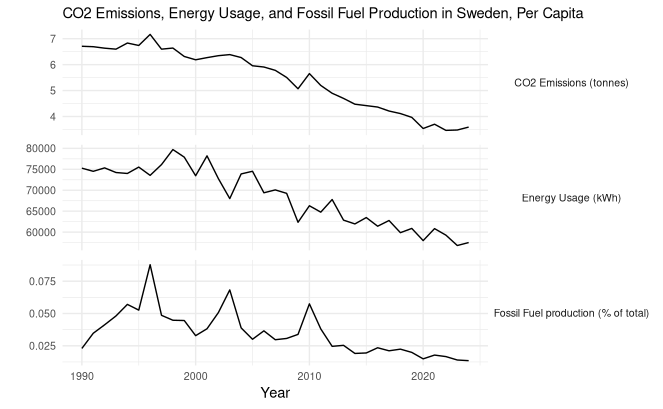
Figure 1: Example of the data.
The posterior of $\beta_3$ has shows that $E[\beta_3] = 0.29$ with a 95% credible interval of $[0.22, 0.35]$. The hypothesis test shows that the probability of $P(\beta_3 = 0 | \text{data}) = 0$ while $P(\beta_3 \geq 0 | \text{data}) = 1$. However, when looking at regional variability accounted for with regression parameter $b_{3j}$ (see Figure 2), the reality is that although we may see an overall positive global correlation, this does not necessarily extend to every country.
![Figure 2: Regional interaction effect $b_{3j}$ for each region, including uncertainties, in a dot-whisker plot. The red line shows $E[\beta_3] = 0.29$, the mean global effect.](/images/bayesian_hierarhical_dot_whisker.png)
Figure 2: Regional interaction effect $b_{3j}$ for each region, including uncertainties, in a dot-whisker plot. The red line shows $E[\beta_3] = 0.29$, the mean global effect.
The result for global effect parameter $\beta_3$ suggests that reducing fossil fuel share in the energy mix could decouple energy usage from CO2 emissions. However, the large variability and uncertainty at the regional level, with some regions/countries even showing opposite correlation, highlights the complexity of drawing definitive conclusions. Improvements could be: accounting for the temporal structure in the data. Also, some regions had limited data available which means large uncertainties, with many of those so large that the null-hypothesis could not be rejected on a regional level. Finally, it is important to highlight that the interaction term is agnostic in terms of causality and merely confirms a joint effect. It does not mean that lower fossil fuel share truly causes the decoupling of energy usage and CO2 emissions.