1D entropic rubber band - Monte Carlo re-weighting techniques

Tip

The git repository, including source code and more detailed documentation, is available here.

Reflection Link to heading

This project explores the statistical simulation of a simple 1D rubber band as a chain of links. It was intended for exploring Monte Carlo simulations and particularly re-weighting techniques.

Theory Link to heading

In statistical terms we can think of the rubber band as a series of fixed-length segments, which have a positive or negative direction. Then, a rubber band of $N$ segments or ’links’ has $n^+$ positive and $n^-$ negative links. The total length $L$ is then

$$L = a(2n^+ - N )$$

With no force applied corresponds to a random assignment which means that $E[L] = 0$.

There are many microstates which correspond to one macrostate of $L$, namely

$$ \Omega(N, n^+) = \binom{N}{n^+} = \frac{N!}{n^+!(N-n^+)!} $$

with this, we have that the true distribution of lengths will be

$$P(L) = \Omega(N, n)/2^N$$

Results Link to heading

Here follows a brief display of the results. Interpretation is in each figure caption.

Rubber band with no force Link to heading

As a sanity test, the first task consisted of simply generating a rubber band with no force applied.

Figure 1: Histogram of sampled lengths for $M=10^6$ samples of a rubber band consisting of $N=100$ length $a=1$ links. $P(L) = \Omega(N, n)/2^N$ represents the true distribution of lengths for a given $N$ and $n=(N+L/a)/2$. $\hat{P}(L)$ represents the normalised histogram for lengths $L$ of the sampled rubber bands. The $\chi^2$ test was done for all bins with more than 5 counts, and shows good agreement between theory and sample. 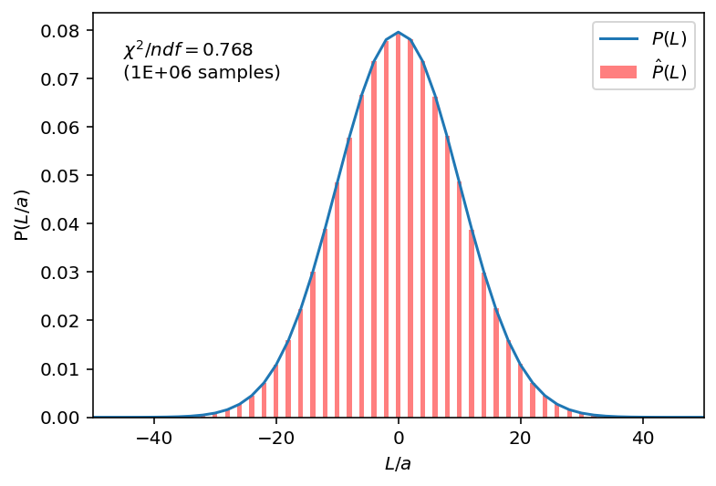— **Figure 1:** Histogram of sampled lengths for $M=10^6$ samples of a rubber band consisting of $N=100$ length $a=1$ links. $P(L) = \Omega(N, n)/2^N$ represents the true distribution of lengths for a given $N$ and $n=(N+L/a)/2$. $\hat{P}(L)$ represents the normalised histogram for lengths $L$ of the sampled rubber bands. The $\chi^2$ test was done for all bins with more than 5 counts, and shows good agreement between theory and sample.

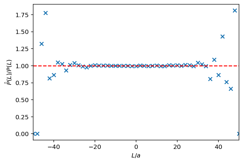
Figure 2: $P(L)/\hat{P}(L)$ for various lengths $L/a$. As expected, the ratio is close to $1$ around $L=0$ where we have sufficient statistics. This latter statement is not true at the tails, where we see the sample probability start to diverge from the true probability. — **Figure 2:** $P(L)/\hat{P}(L)$ for various lengths $L/a$. As expected, the ratio is close to $1$ around $L=0$ where we have sufficient statistics. This latter statement is not true at the tails, where we see the sample probability start to diverge from the true probability.

Rubber band with force (weighting) Link to heading

Suppose we want to apply a force $f$. Obviously one way to get a updated $\hat{P}(L)$ is to resample with some force applied. But this is inefficient, if we already have some previous sample. One way to avoid having to resample is weighting the original unbiased distribution by applying a Boltzmann weight to each microstate

$$\omega = \exp{(\beta fL)}, \quad \beta = 1/k_BT.$$

The new true distribution then becomes

$$ P_f(L) = \frac{\Omega(N, n) e^{\beta f L}}{Z(f)}, \quad Z(f) = \sum_L \Omega(N, n) e^{\beta f L} $$

Figure 3: Histograms for the weighted distributions with $k_BT=a=1$. In green is the original, unbiased distribution $\hat{P}(L)$. Red and blue show the sampled and true distributions with applied weights, according to the description above this figure. What we see is that weighting only works with good statistics. When the force $f$ causes $\hat{P}(L)$ to shift too much beyond the original distribution, the lack of statistics (available samples to weight) causes incorrect results. The figure also shows $\mu_{eff}$, the effective percentage of samples used in the weighted distribution, for each force applied. — **Figure 3:** Histograms for the weighted distributions with $k_BT=a=1$. In green is the original, unbiased distribution $\hat{P}(L)$. Red and blue show the sampled and true distributions with applied weights, according to the description above this figure. What we see is that weighting only works with good statistics. When the force $f$ causes $\hat{P}(L)$ to shift too much beyond the original distribution, the lack of statistics (available samples to weight) causes incorrect results. The figure also shows $\mu_{eff}$, the effective percentage of samples used in the weighted distribution, for each force applied.

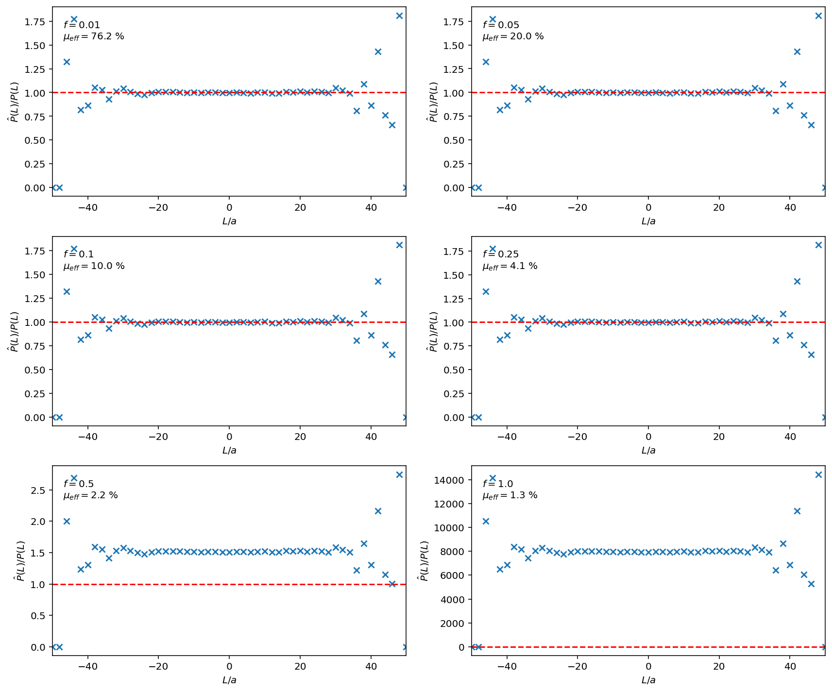
Figure 4: Ratio plots for the weighted distributions. We see that the sampled distribution after weighting becomes unrepresentative of the true underlying distribution for higher forces $f$. — **Figure 4:** *Ratio plots for the weighted distributions. We see that the sampled distribution after weighting becomes unrepresentative of the true underlying distribution for higher forces $f$.*

Figure 5: A plot of force against $\mu_{eff}$. Clearly one can see that effective sample size decreases exponentially with increasing $f$, so the weighting technique, while very efficient, only work with sufficient overlap between the source and target distributions, in this case, small $f$. — **Figure 5:** A plot of force against $\mu_{eff}$. Clearly one can see that effective sample size decreases exponentially with increasing $f$, so the weighting technique, while very efficient, only work with sufficient overlap between the source and target distributions, in this case, small $f$.

Resampling and approximating expected length as function of force Link to heading

When weighting breaks down we must resample. How can one implement this? One way is to bias the sampling. Instead of $p_+ = p_- = 0.5$, we let $p_+$ depend on the force $f$. This is given by

$$p_+(f) = \frac{w_+}{w_+ + w_-} = \frac{e^{\beta f a}}{e^{\beta f a} + e^{-\beta f a}} = \frac{1}{2}(1 + \tanh(\beta f a))$$

and then of course $p_-(f) = 1-p_+(f)$. One can see here that when $f=0$ the above reduces to the simple $p_+ = p_- = 0.5$. Now, we then have that the expected length for some applied force is

$$ \langle L \rangle (f) = N a \tanh(\beta fa).$$

If $\beta fa \ll 1$, the small force approximation

$$\langle L \rangle (f ) \approx \frac{Nfa^2}{k_BT}$$

may be used. In this final simulation, we seek to find out how the mean lengths $L$ from biased sampling according to the force-dependent $p_+(f)$ align with the theoretical expected value and the small force approximation.

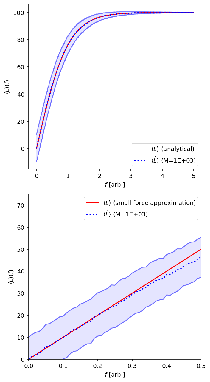
Figure 6: $\langle L \rangle (f)$ for various forces $f$. We have $M=10^3$ samples for each $f$, with $k_BT=a=1$ and $N=100$, which gives a $k_{eff}$ of $100$. The analytical formulas are in red and are described above this figure. We can see excellent agreement with the analytical $\langle L \rangle(f)$ across a large range of $f$. However, the small force approximation in the lower figure starts to diverge at $f > 0.3$. A linear fit to $\langle \hat{L} \rangle(f<0.3)$ gives us an estimated $k_{eff} \approx 96.93$. 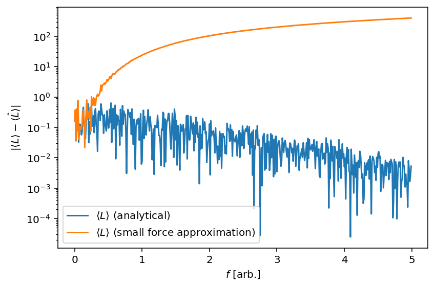— **Figure 6:** $\langle L \rangle (f)$ for various forces $f$. We have $M=10^3$ samples for each $f$, with $k_BT=a=1$ and $N=100$, which gives a $k_{eff}$ of $100$. The analytical formulas are in red and are described above this figure. We can see excellent agreement with the analytical $\langle L \rangle(f)$ across a large range of $f$. However, the small force approximation in the lower figure starts to diverge at $f > 0.3$. A linear fit to $\langle \hat{L} \rangle(f<0.3)$ gives us an estimated $k_{eff} \approx 96.93$.

Figure 7: To clarify Figure 6, the absolute difference between the sampled $\langle \hat{L} \rangle(f)$ and $\langle L \rangle(f)$ as well as $\langle L \rangle(f)$ with the small force approximation. We can very clearly see that the small force approximation breaks down around an $f$ of $0.3-0.4$. — **Figure 7:** To clarify Figure 6, the absolute difference between the sampled $\langle \hat{L} \rangle(f)$ and $\langle L \rangle(f)$ as well as $\langle L \rangle(f)$ with the small force approximation. We can very clearly see that the small force approximation breaks down around an $f$ of $0.3-0.4$.